Ch 2. Autoregressive Models¶

约 322 个字 3 张图片预计阅读时间 1 分钟

Representation¶

The fundamental goal is to model the joint distribution \(p(\mathbf{x})\) of \(n\)-dimensional data \(\mathbf{x} \in \{0,1\}^n\).

The Chain Rule Decomposition¶

Using the probability chain rule, any joint distribution can be decomposed into a product of conditionals:

\[p(\mathbf{x}) = \prod_{i=1}^{n} p(x_i \mid \mathbf{x}_{<i})\]

where \(\mathbf{x}_{<i} = [x_1, \dots, x_{i-1}]\).

The Autoregressive Property¶

A model is autoregressive if it respects a fixed ordering of variables. Each variable \(x_i\) depends only on its predecessors.

While a tabular representation of these conditionals leads to exponential space complexity \(O(2^n)\), ARMs use parameterized functions to keep the complexity manageable.

Model Architectures¶

The evolution of ARMs is a journey from simple linear maps to efficient neural weight-sharing.

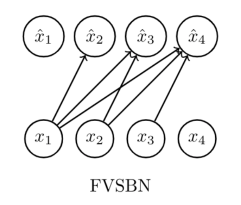
FVSBN (Fully Visible Sigmoid Belief Network)¶

The simplest case where each conditional is a Logistic Regression:

\[ f_i(\mathbf{x}_{<i}) = \sigma\left( \alpha^{(i)}_0 + \sum_{j=1}^{i-1} \alpha^{(i)}_j x_j \right) \]

Complexity: \(O(n^2)\) parameters.

MLP¶

Enhances expressivity by using an independent MLP for each \(i\):

\[ \begin{aligned} \mathbf{h}_i &= \sigma(\mathbf{A}_i \mathbf{x}_{<i} + \mathbf{c}_i), \\ f_i &= \sigma(\boldsymbol{\alpha}^{(i)} \mathbf{h}_i + b_i), \end{aligned} \]

where \(\theta_i = \{\mathbf{A}_i \in \mathbb{R}^{d \times (i-1)}, \mathbf{c}_i \in \mathbb{R}^d, \boldsymbol{\alpha}^{(i)} \in \mathbb{R}^d, b_i \in \mathbb{R}\}\).

Complexity: \(O(n^2 d)\) parameters, where \(d\) is the hidden layer size.

NADE (Neural Autoregressive Density Estimator)¶

Do weight sharing:

\[\mathbf{h}_i = \sigma(\mathbf{W}_{.,<i} \mathbf{x}_{<i} + \mathbf{c}),\]

where \(\theta = \{\mathbf{W} \in \mathbb{R}^{d \times n}, \mathbf{c} \in \mathbb{R}^d, \{\boldsymbol{\alpha}^{(i)} \in \mathbb{R}^d\}_{i=1}^n, \{b_i \in \mathbb{R}\}_{i=1}^n\}\).

Complexity: \(O(nd)\) parameters.

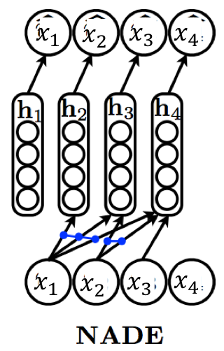
Hidden states can be computed via a recursive update:

\[ \begin{aligned} \mathbf{h}_i &= \sigma(\mathbf{a}_i), \\ \mathbf{a}_{i+1} &= \mathbf{a}_i + \mathbf{W}_{[.,i]} x_i. \end{aligned} \]

Learning & Inference¶

Maximum Likelihood Estimation (MLE)¶

Learning is framed as minimizing the Forward KL Divergence \(D_{\text{KL}}(p_{\text{data}} \parallel p_{\theta})\):

\[ \min_{\theta \in \Theta} D_{\text{KL}}(p_{\text{data}} \parallel p_{\theta}) = \mathbb{E}_{\mathbf{x} \sim p_{\text{data}}} \left[ \log p_{\text{data}}(\mathbf{x}) - \log p_{\theta}(\mathbf{x}) \right], \]

which is mathematically equivalent to maximizing the Log-Likelihood:

\[ \max_{\theta \in \Theta} \mathbb{E}_{\mathbf{x} \sim p_{\text{data}}} \left[ \log p_{\theta}(\mathbf{x}) \right], \]

and (if i.i.d.):

\[ \max_{\theta} \mathcal{L}(\theta \mid \mathcal{D}) = \frac{1}{|\mathcal{D}|} \sum_{\mathbf{x} \in \mathcal{D}} \sum_{i=1}^{n} \log p_{\theta_i}(x_i \mid \mathbf{x}_{<i}). \]

Optimization: Solved via Stochastic Gradient Ascent (or Descent on the Negative Log-Likelihood) using Autograd.

\[ \theta^{(t+1)} = \theta^{(t)} + r_t \nabla_{\theta} \mathcal{L}(\theta^{(t)} \mid \mathcal{B}_t) \]

Tip

Forward KL Property: "Zero-avoiding," forcing the model to cover all modes of the data (ensuring diversity but potentially causing hallucinated samples).

Inference Tasks¶

Density Estimation: Parallelizable. We can compute all \(p(x_i | \mathbf{x}_{<i})\) simultaneously if the input \(\mathbf{x}\) is known.
Sampling: Sequential. Must sample \(x_1\), then \(x_2\) given \(x_1\), and so on. \(O(n)\).